Understanding and Computing the Hilbert Regularity

When attacking AOCs using Gröbner bases, the most relevant question is: how complex is the Gröbner basis computation? One commonly used estimation is based on the degree of regularity. Intuitively, the degree of regularity is the degree of the highest-degree polynomials to appear during the Gröbner basis computation. (Whether this metric is good for estimating the AOC's security is a different matter.)

Unfortunately, different authors define the term “degree of regularity” differently. In this post, I use the understanding of Bardet et al. [1,2], which coincides with the well-defined Hilbert regularity.

I first introduce the required concepts, and then make them more tangible with some examples. Lastly, there is some sagemath code with which the Hilbert regularity can be computed.

Definition of the Hilbert Regularity

Let $\mathbb{F}$ be some field, $R = \mathbb{F}[x_0, \dots, x_{n-1}]$ a polynomial ring in $n$ variables over $\mathbb{F}$ , and $I \subseteq R$ a polynomial ideal of $R$ .

The affine Hilbert function of quotient ring $R/I$ is defined as $${}^a\textsf{HF}_{R/I}(s) = \dim_\mathbb{F}\!\left(R_{\leqslant s} \middle/ I_{\leqslant s}\right).$$ For some large enough value $s_0$ , the Hilbert function of all $s \geqslant s_0$ can be expressed as a polynomial in $s$ . 🛈 For a general treatment of the how? and why?, have a look at the excellent book “Ideals, Varieties, and Algorithms,” [3] in particular Chapter 9, §2, Theorem 6, and Chapter 9, §3. The examples in this post hopefully shed some light, too. This polynomial, denoted ${}^a\textsf{HP}_{R/I}(s)$ , is called Hilbert polynomial. By definition, the values of the Hilbert function and the Hilbert polynomial coincide for values greater than $s_0$ .

The Hilbert regularity is the smallest $s_0$ such that for all $s \geqslant s_0$ , the evaluation of the Hilbert function in $s$ equals the evaluation of the Hilbert polynomial in $s.$

By the rank-nullity theorem, we can equivalently write the Hilbert function as $${}^a\textsf{HF}_{R/I}(s) = \dim_\mathbb{F}\! \left( R_{\leqslant s} \right) - \dim_\mathbb{F}\! \left( I_{\leqslant s}\right).$$ This is a little bit easier to handle, because we can look at $R$ and $I$ separately and can ignore the quotient ring $R/I$ for the moment. By augmenting $R$ with a graded monomial order, like degrevlex, we can go one step further and look at leading monomials $\textsf{lm}$ only: the set $\{ \textsf{lm}(f) \mid f \in I, \deg(f) \leqslant s \}$ is a basis for $I_{\leqslant s}$ as an $\mathbb{F}$ -vector space. 🛈 See [3, Chapter 9, §3, Proposition 4] for a full proof. Meaning we don't even need to look at $I$ , but can restrict ourselves to the ideal of leading monomials $\langle \textsf{lm}(I) \rangle$ . $${}^a\textsf{HF}_{R/I}(s) = \dim_\mathbb{F}\!\left(R_{\leqslant s}\right) - \dim_\mathbb{F}\!\left( \langle \textsf{lm}(I) \rangle_{\leqslant s}\right).$$

One way to get a good grip on $\langle I \rangle$ is through reduced Gröbner bases. A Gröbner basis $G$ for ideal $I$ is a finite set of polynomials with the property $\langle G \rangle = \langle I \rangle$ and, more relevant right now, $\langle \textsf{lm}(G) \rangle = \langle \textsf{lm}(I) \rangle.$ This means it's sufficient to look at (the right combinations) of elements of $\textsf{lm}(G).$ This, in turn, is more manageable because $G$ always has finitely many elements, but $I$ might not.

Example: 0-Dimensional Ideal

Let's start with a super simple polynomial system: $$G = \{x^6, x^2y^2, y^5\} \subseteq \mathbb{F}[x,y], \quad I = \langle G \rangle$$ for some finite field $\mathbb{F}.$ This is a zero-dimensional, monomial (thus homogeneous) ideal. That's about as special as a special case can get. Note that here, we have $I = \langle \textsf{lm}(I) \rangle$ , but this doesn't generally hold. Dealing with a super-special case also means that the Hilbert polynomial is relatively boring, but that's fine for starting out. $G$ is the reduced Gröbner basis for $I$ , and we'll use its elements to help computing the Hilbert function.

A benefit of ideals in two variables is: we can draw pictures.

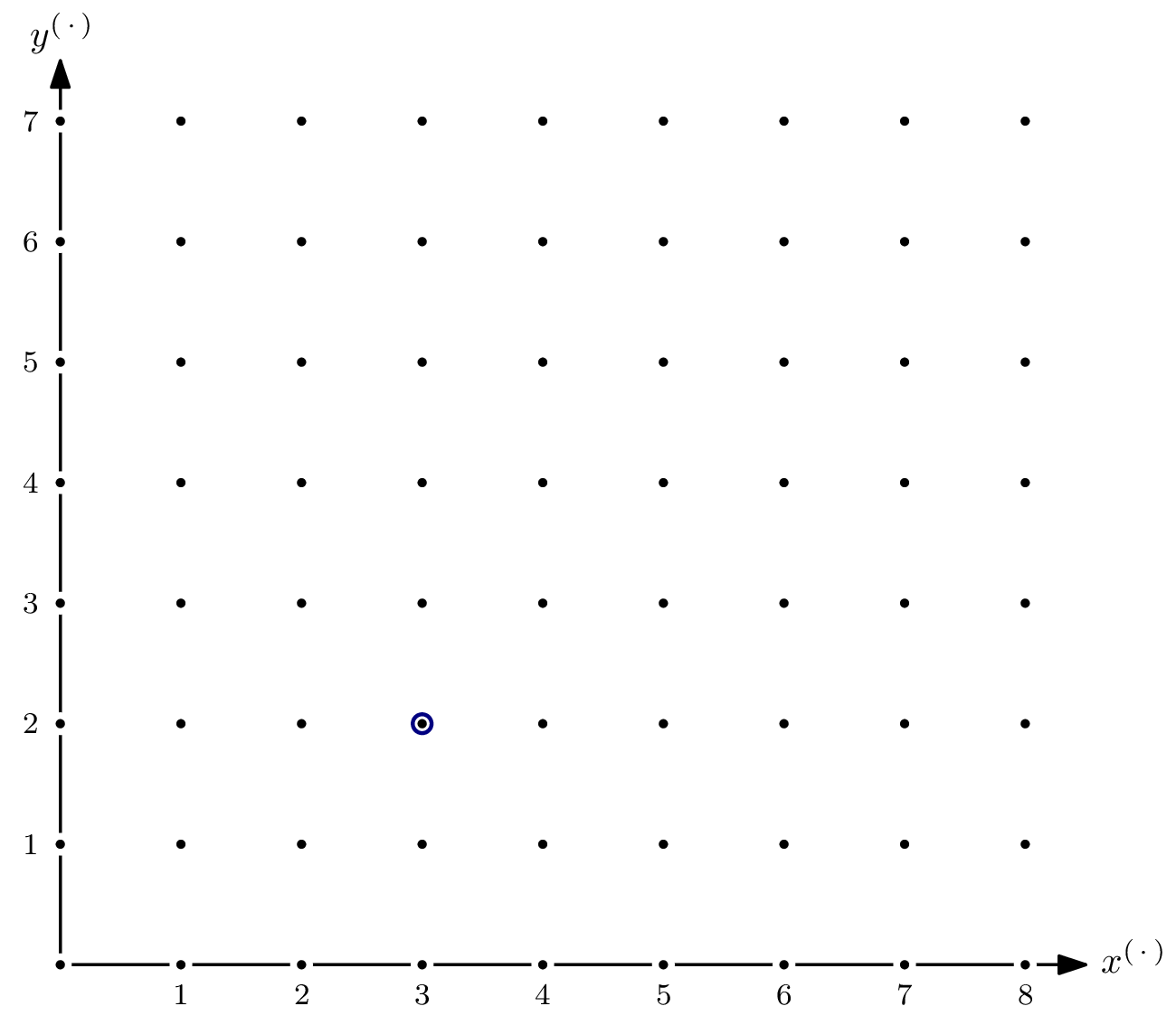
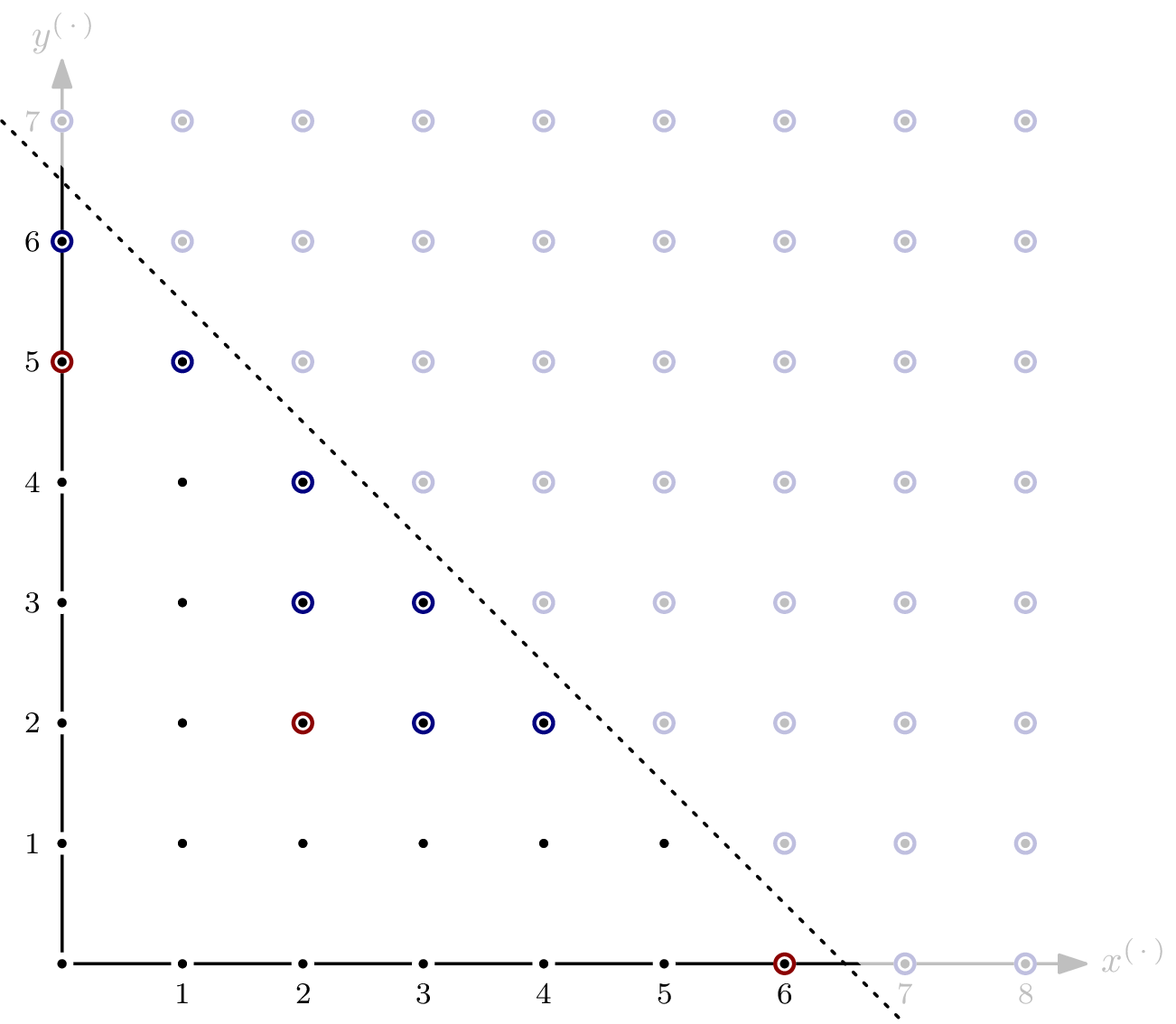
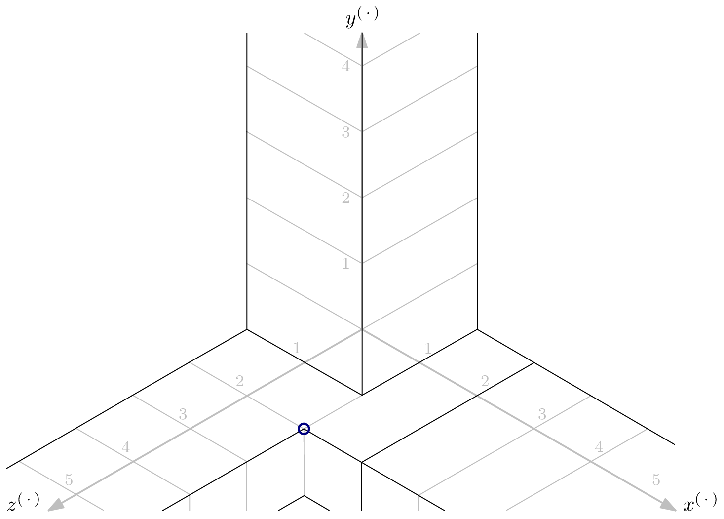
This is what the monomials of $\mathbb{F}[x,y]$ as an $\mathbb{F}$ -vector space look like. Well, at least the part $\{x^ay^b \mid a \leqslant 8, b \leqslant 7 \}.$ After all, $\mathbb{F}[x,y]$ as an $\mathbb{F}$ -vector space has infinite dimension. I have (arbitrarily) highlighted $x^3y^2,$ i.e., coordinate (3,2), to give a better understanding of what the picture means.

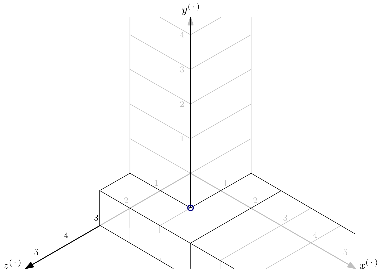
Since $I$ is a monomial ideal, we can highlight every element in $I$ . The circles of the elements of the Gröbner basis $G$ are red. The zig-zig pattern of the boundary between $x^ay^b \in I$ and $x^ay^b \notin I$ is inherent, and generalizes to higher dimensions, i.e., more variables. Because of the zig-zagging, the set of monomials not in $\langle \textsf{lm}(I) \rangle$ is referred to as staircase of $I.$

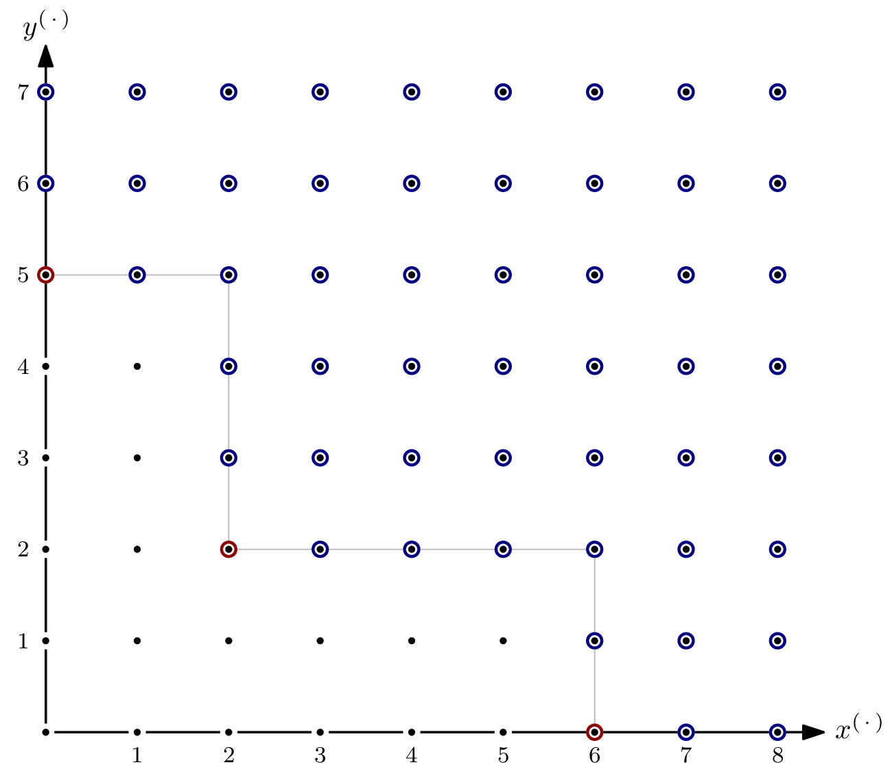
Let's start computing the Hilbert function for $R/I.$ The $\mathbb{F}$ -vector space dimensions of $R_{\leqslant s}$ and $I_{\leqslant s}$ are simply the number of monomials in $R$ respectively $I$ with degree $\leqslant s.$ Getting those numbers is easy – it amounts to counting dots in the picture! For example, for $s=2,$ , we have ${}^a\textsf{HF}_{R/I}(2)=5-0=5:$

No monomial of total degree less than or equal to 2 is in $I$ , so computing the Hilbert function is a little bit boring here.

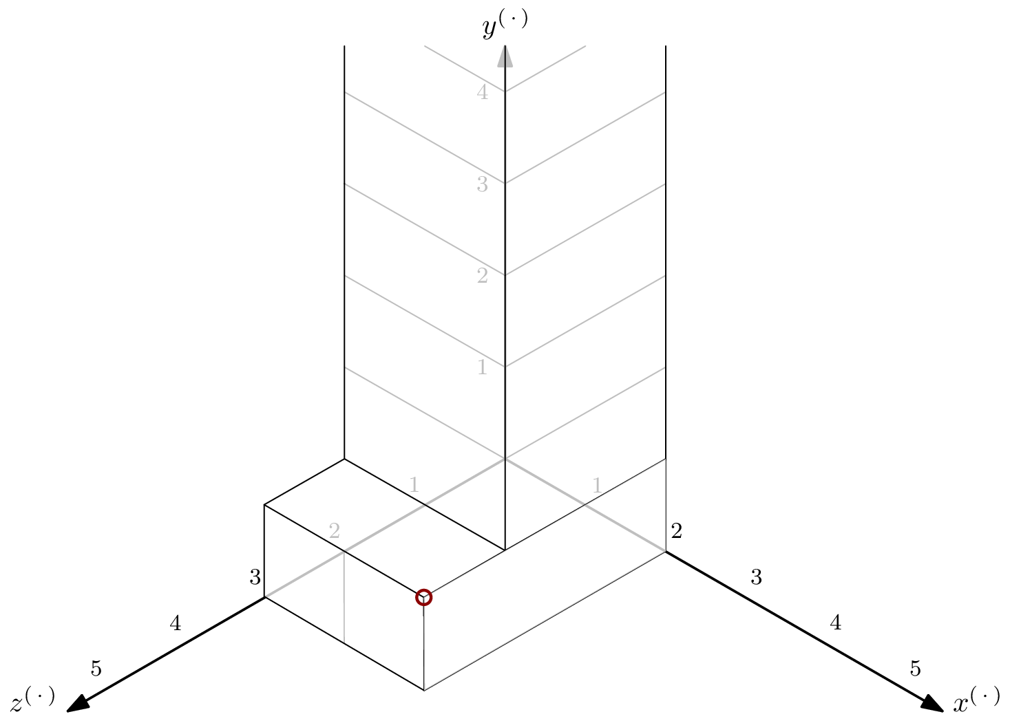
The value of the Hilbert function ${}^a\textsf{HF}_{R/I}(5)$ is more interesting: some monomials of degree $\leqslant 5$ are indeed elements of $I$ , and thus $\dim I_{\leqslant 5}$ is not 0 but 4. In particular, we have ${}^a\textsf{HF}_{R/I}(5)=21 - 4=17.$ For $s=6,$ we have ${}^a\textsf{HF}_{R/I}(6)=28-10=18:$

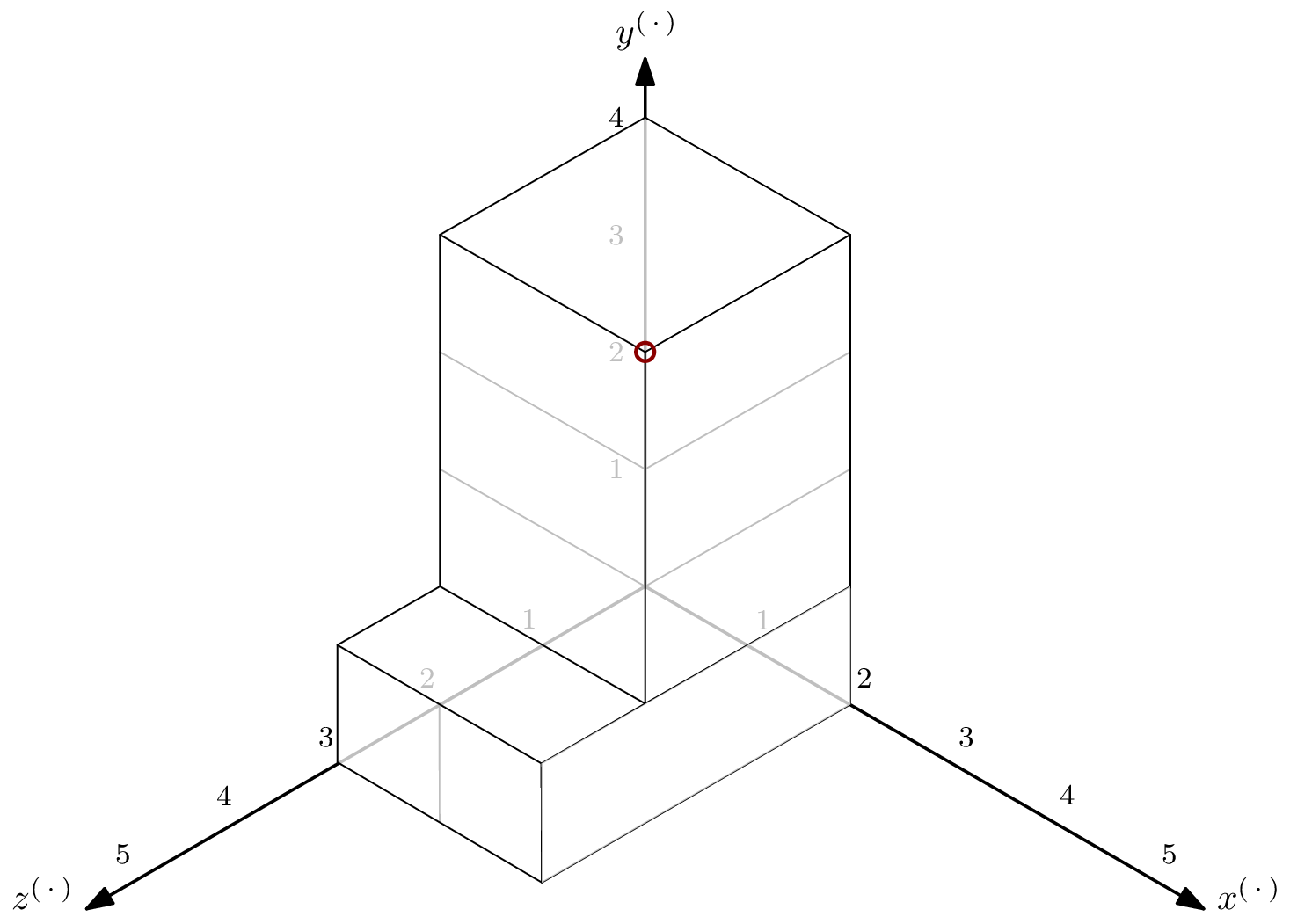
From this point forward, increasing $s$ will not change the value of the Hilbert function – the dimension of $I_{\leqslant s}$ as an $\mathbb{F}$ -vector space grows with the same rate as the dimension of $R_{\leqslant s}$ , since all monomials not in $I$ are of lesser total degree. Expressed differently, all monomials above the line are elements of both $I$ and $R$ – the values of the Hilbert function doesn't change by increasing $s.$

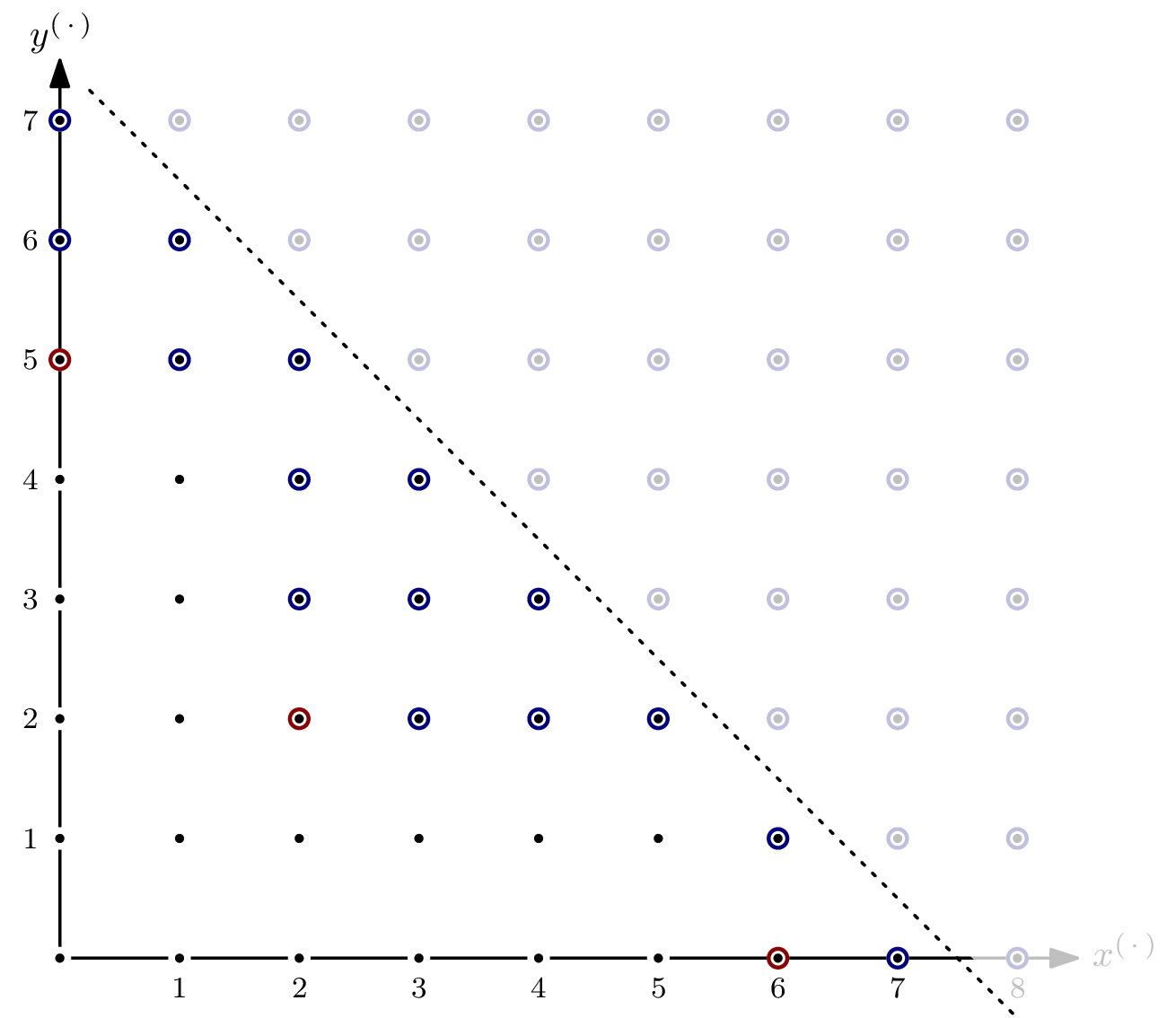
From this, two things follow:

1. The Hilbert polynomial of $R/I$ is the constant 18. (That's why I said it's relatively boring. A more interesting case follows.)
2. The Hilbert regularity of $R/I$ is 6, since ${}^a\textsf{HF}_{R/I}(s) = {}^a\textsf{HP}_{R/I}(s)$ for all $s \geqslant 6.$

Example: Ideal of Positive Dimension

As hinted at above, whether or not $I$ is a monomial ideal does not matter for computing the Hilbert function or the Hilbert polynomial, because $\textsf{lm}(I)$ behaves exactly the same. What does matter, though, is the dimension of $I.$ In the previous example, $I$ was of dimension 0, and the Hilbert polynomial of $R/I$ was a constant. That's not a coincidence.

Even though the ideal spanned by the polynomial system modelling an AOC will usually be zero-dimensional, it's interesting to see what happens if it isn't. Let's take $G = \{x^4y^3, x^2y^5\} \subseteq \mathbb{F}[x,y]$ and $I = \langle G \rangle.$

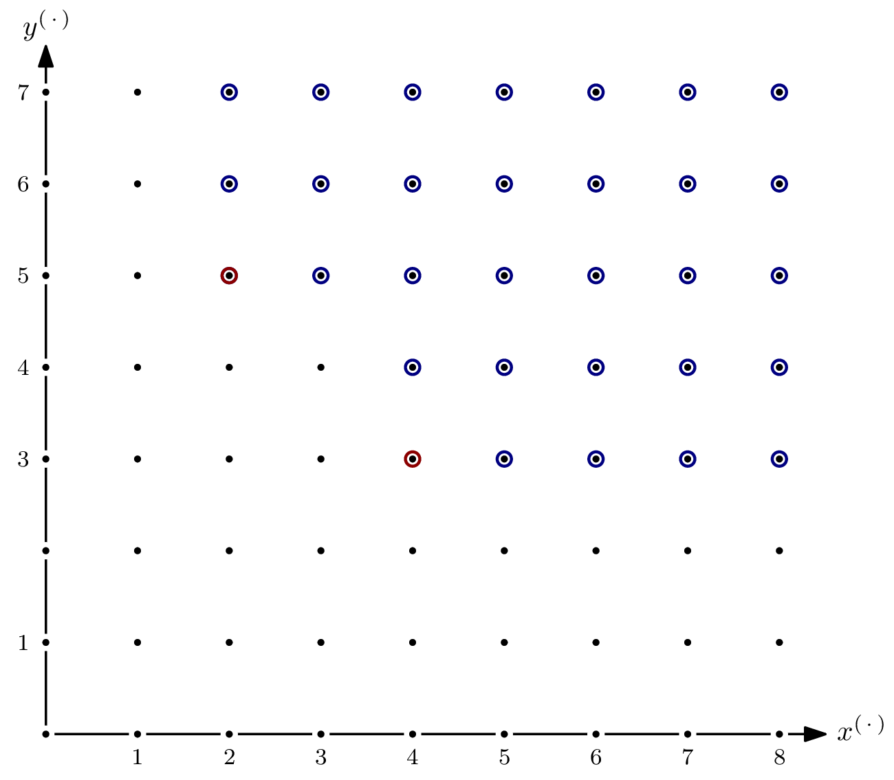
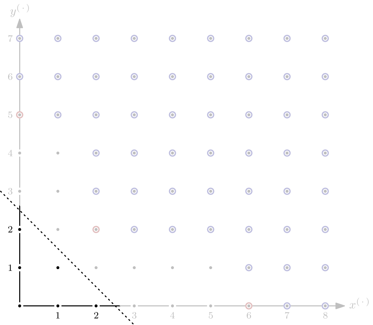
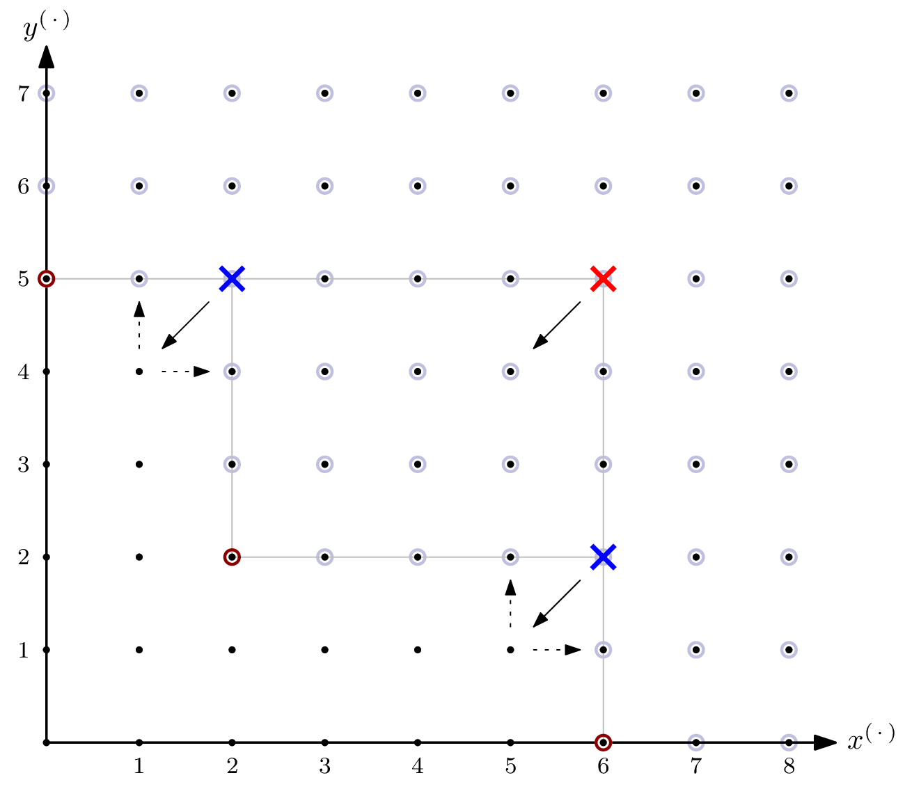
As you can see, there are parts of the staircase that extend to infinity. That's a direct consequence of $I$ having positive dimension, or, equivalently, variety $V(I)$ not having finitely many solutions. In the picture below, I've indicated the staircase's five subspaces of dimension $1$ by dashed, gray lines.

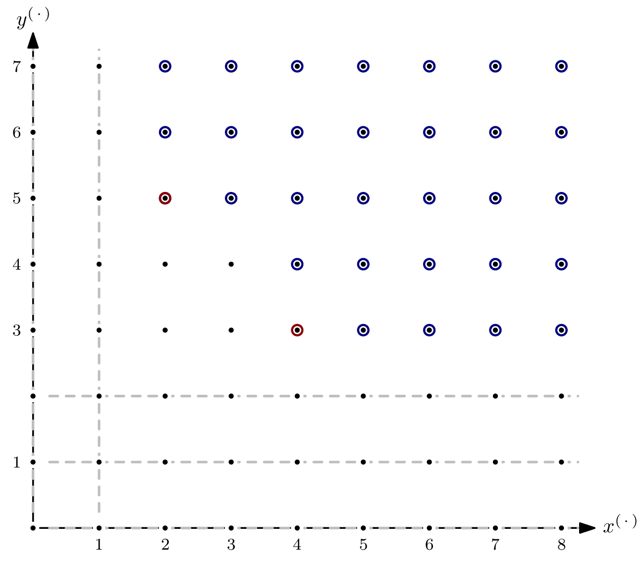
For the Hilbert function, only monomials in $I$ of degree $\leqslant s$ are relevant. For each of the five subspaces, we can express the matching number of elements as a polynomial in $s.$

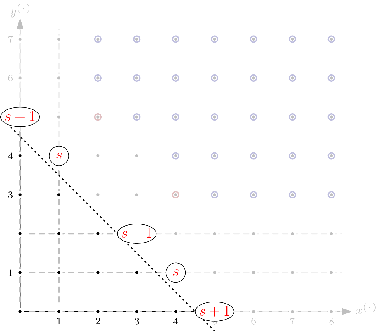
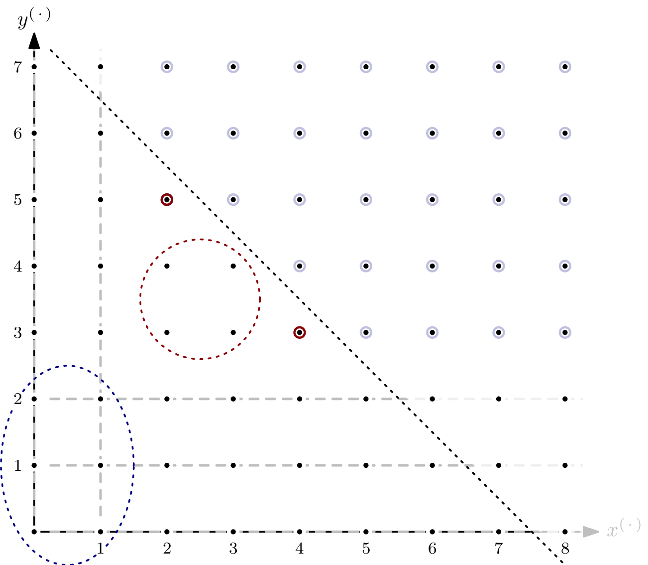
The sum of these five polynomials is $5s+1,$ which corresponds to the total number of monomials in the staircase of $I$ of degree $\leqslant s$ that lie in the staircase's 1-dimensional subspaces – except that some elements are counted more than once. Since the intersection of two orthogonal 1-dimensional subspaces is of dimension $0$ , we can simply add a constant correction term. 🛈 For ideals with more than two variables, we generally need to add correction terms of higher dimension, corresponding to polynomial summands of degree higher than 0.

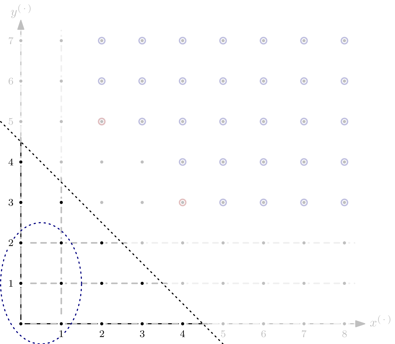
Adding the correction term of $-6$ gives $5s-5$ as a (preliminary) Hilbert polynomial for $I.$ We're not completely done yet: for $s > 4$ , there are monomials not in $I$ that are also not in any of the 1-dimensional subspaces – for example $x^3y^3.$ Of those, we only have finitely many. In the example, it's 4.

After adding the second correction term, we have ${}^a\textsf{HP}_{I/R}(s)=5s-1$ .

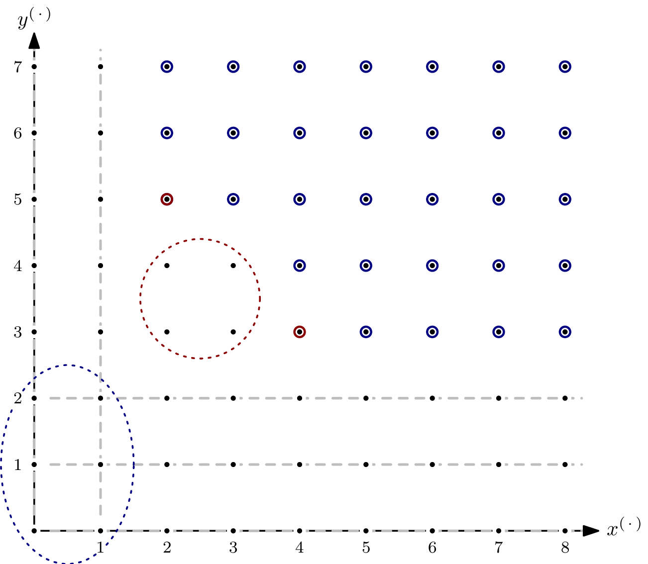
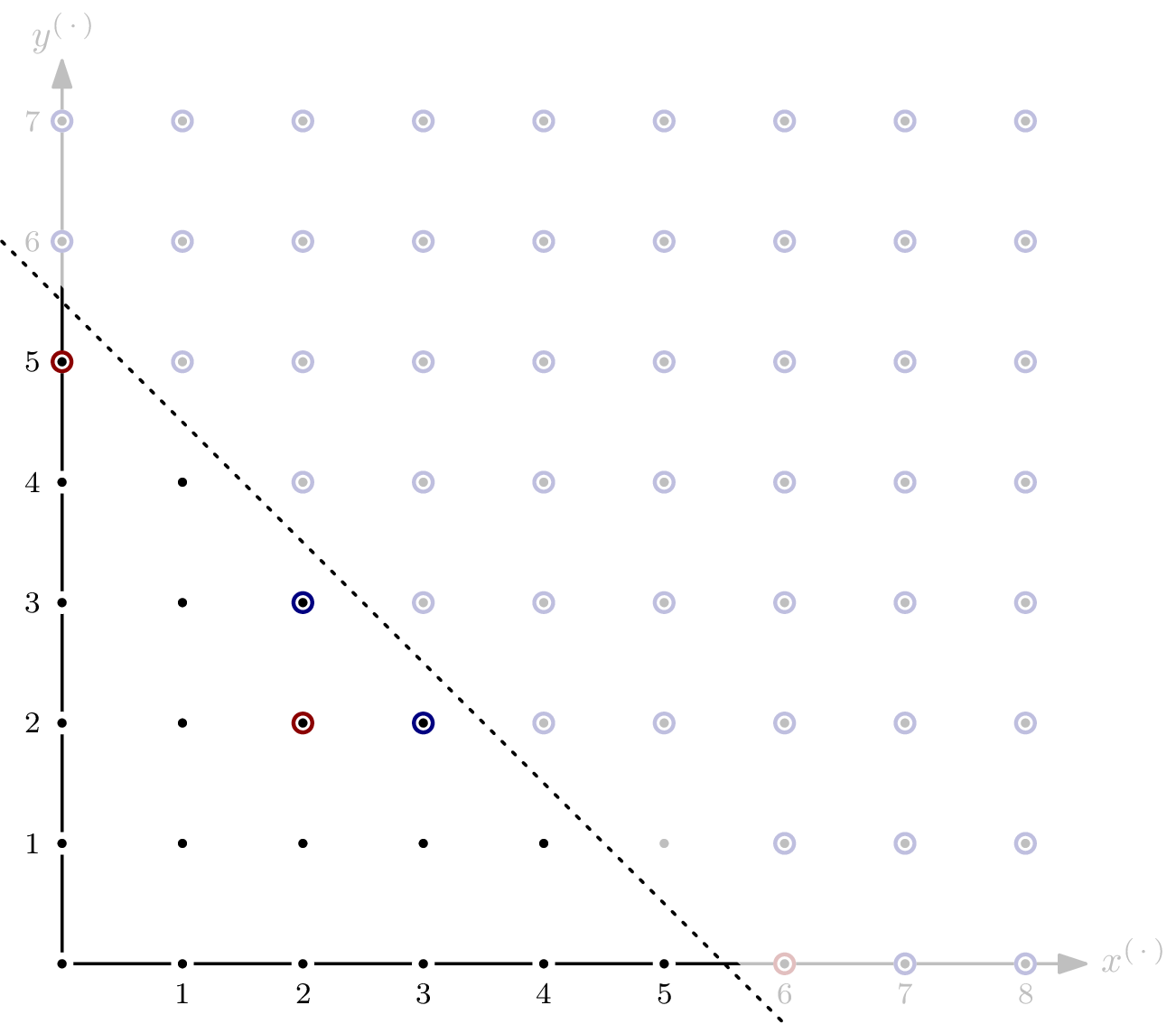
By finding the Hilbert polynomial, we also computed the Hilbert regularity of $R/I:$ it's $7.$ In other words, for $s\geqslant 7,$ we have $\dim_\mathbb{F}(R/I) = {}^a\textsf{HF}_{R/I}(s) = {}^a\textsf{HP}_{R/I}(s) = 5s-1.$

This coincides with the distance of the closest diagonal 🛈 Generally speaking, the diagonal is a hyperplane. such that all “overlapping” as well as all zero-dimensional parts of the staircase are enclosed – the red and blue dashed circles, respectively, in above picture.

More Variables, More Dimensions

The intuition of the 2-dimensional examples above translate to higher dimensions: find the most distant corner of the blue circle – the parts where positive-dimensional subspaces of the variety overlap – and the red circle – the variety's part of dimension zero – and take the distance of the farther of these two corners as the Hilbert regularity. However, finding the corners becomes less trivial. Let me demonstrate with a staircase consisting of three “tunnels” that we'll successively modify.

Above staircase is defined by $G=\{x^2y, x^2z^3, yz^2\}.$ No monomials exist in the red bubble – every point is part of a subspace of dimension 1. The blue corner is the monomial defining the enclosing space of the parts where positive-dimensional subspaces overlap. It coincides with the least common multiple (lcm) of the three elements of $G,$ namely $m=x^2yz^3.$ The Hilbert regularity can be read off from $m\!$ : the hyperplane's required distance is $\deg(x^{(2-1)}y^{(1-1)}z^{(3-1)})=3.$

That was easy enough. Let's take a look at $G' = \{x^2y, yz^2, z^3\}.$ The staircase looks similar, with the exception for the “$z$ -tunnel.”

Even though $m$ from above is still on the “border” of $\langle G' \rangle,$ just as it was for $\langle G \rangle,$ it no longer defines the enclosing space we're looking for. Note that the lcm of the elements in $G'$ is still $m,$ but the Hilbert regularity is now defined by the lcm of only two elements, $x^2y$ and $yz^2,$ giving $m' = x^2yz^2.$ The Hilbert regularity has changed to $2.$

Let's modify the staircase a little bit more, and look at $G^\dagger = \{x^2, yz^2, z^3\}.$

he Hilbert regularity can once again be found by looking at $m = x^2yz^3,$ but the reason has changed. This time around, $m$ is the most distant corner of the volume enclosing all monomials not appearing in positive-dimensional subspaces of the variety – that's the red bubble from before. And since only one “tunnel” remains, there's no more overlap in positive-dimensional subspaces – the blue bubble, and with it the blue dot, have disappeared. Note that $m$ is once again the lcm of the three elements of $G^\dagger.$ The Hilbert regularity is now again 3.

For completeness sake, let's close off the last of the tunnels by adding $y^4$ to $G^\dagger.$ Monomial $m^\dagger = x^2y^4z^2,$ being the lcm of $x^2,$ $yz^2,$ and $y^4,$ is the Hilbert regularity-defining corner. The Hilbert regularity for $G^\dagger$ is 5.

Computing the Regularity in sagemath

After having understood the Hilbert regularity, it's time to throw some sagemath at the problem. Below, you can find two approaches. The first uses the staircase, like in the examples above. The second is based on the Hilbert series, which is explained further below.

The nice-to-visualize geometric approach

Using the geometric intuitions from above, we can compute the Hilbert regularity by finding all of the staircase's corners. The code below only works for ideals of dimension 0 🛈 Technically, the code works for any dimension ≤ 0, i.e., if there are no common solutions to the polynomials in the ideal, it also works. since the polynomial models I do research on are always of that kind.

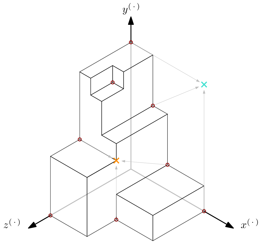
The code computes all lcm's of subsets of size $n$ of the Gröbner basis' leading monomials, which we have determined as the points of interest above. Any such lcm corresponding to a monomial that's flush to one of the 0-planes is ignored as being degenerate – for example, the turquoise cross in below picture. Next, we check if the lcm-monomial is actually a corner of the staircase, by moving one step towards the origin along all axes. If the resulting monomial is in the ideal, it is not in the staircase, and thus not a corner – for example, the red cross in above picture. If, from the moved-to monomial, moving one step along any axis crosses the border of the staircase, we found a corner – for example, both of the blue crosses in above picture, but not the orange cross in the picture below. The distance of the furthest such corner corresponds to the Hilbert regularity.

With those pictures in mind, following the code should be fairly doable:

import combinations
def hilbert_regularity_staircase(I):
    '''
    Compute the Hilbert regularity of R/I where R = I.ring() and I.dimension() <= 0.
    This is done by iterating through all n-tuples of the Gröbner basis' leading monomials,
    computing their lcm, then determining if that lcm is actually a corner of the staircase.
    The corner that is the furthest from the origin determines the Hilbert regularity.
    '''
    if I.dimension() > 0:
        raise NotImplementedError(f"Ideal must be of dimension 0 or less, but has dim {I.dimension()}.")
    gens = I.ring().gens() # all variables
    n = len(gens)
    xyz = reduce(operator.mul, gens, 1)
    gb_lm = [f.lm() for f in I.groebner_basis()]
    I_lm = Ideal(gb_lm)
    hil_reg = 0
    for lms in combinations(gb_lm, n):
        m = lcm(lms)
        # are we considering a meaningful combination of lm's?
        # i.e., does every variable make an appearance in m?
        if len(m.degrees()) != n or not all(m.degrees()):
            continue
        m = m / xyz # 1 step towards origin along all axes
        assert I.ring()(m) == m.numerator() # no negative exponents, please
        m = I.ring()(m)
        # are we in a corner of the staircase?
        # i.e., not in the ideal, but moving 1 step along any axis, we end up in the ideal?
        if not m in I_lm and all([v*m in I_lm for v in gens]):
            hil_reg = max(hil_reg, m.degree())
    return hil_reg

The rigorous mathematical approach

The Hilbert regularity can also be computed using the Hilbert series. The Hilbert series is the formal power series of the (projective) Hilbert function: 🛈 We can either look at the projective Hilbert function, or equivalently subtract two consecutive values of the affine Hilbert function, as I am doing here. $$\textsf{HS}_{R/I}(t) = \sum_{s=1}^{\infty}({}^a\textsf{HF}_{R/I}(s) - {}^a\textsf{HF}_{R/I}(s-1))t^s$$ The Hilbert series' coefficient of monomial $t^d$ is the number of monomials of degree $d$ 🛈 Unlike before, we only consider equality now! that are in $R$ but not in $I.$ The Hilbert regularity coincides with the degree of the highest-degree consecutive term having positive coefficient.

For example, take $I$ from the very first example again, where we had $G = \{x^6, x^2y^2, y^5\}.$ Evaluating the Hilbert function of $R/I$ gives $(1, 3, 6, 10, 14, 17, 18, 18, \dots).$ The Hilbert series of $R/I$ is $$\textsf{HS}_{R/I}(t) = 1 + 2t + 3t^2 + 4t^3 + 4t^4 + 3t^5 + t^6.$$ And indeed, the sought-for term has degree $6,$ which we have seen to be the Hilbert regularity of $R/I.$

Conveniently, sagemath has a method for computing the Hilbert series of an ideal, albeit only for homogeneous ideals. As we have established above, the Hilbert regularity does not change when looking only at the leading monomials of the ideal's Gröbner basis, which is a homogeneous ideal. Thus, finally, we have a catch-all piece of code for computing the Hilbert regularity.

def hilbert_regularity(I):
    '''
    Compute the Hilbert regularity of R/I using the Hilbert series of R/I.
    '''
    gb_lm = [f.lm() for f in I.groebner_basis()]
    I_lm = Ideal(gb_lm)
    hil_ser = I_lm.hilbert_series()
    hil_reg = hil_ser.numerator().degree() - hil_ser.denominator().degree()
    return hil_reg

Summary

In this post, we have looked at the Hilbert function, the Hilbert polynomial, the Hilbert regularity, and the Hilbert series. For the first two of those, extensive examples have built intuition for what the Hilbert regularity is – and why it is not trivial to compute using this intuition. Instead, the Hilbert series gives us a tool to find the Hilbert regularity fairly easily.

References

1. Magali Bardet, Jean-Charles Faugère, Bruno Salvy, and Bo-Yin Yang. Asymptotic behaviour of the degree of regularity of semi-regular polynomial systems. In Proceedings of MEGA, volume 5, 2005.
2. Alessio Caminata and Elisa Gorla. Solving multivariate polynomial systems and an invariant from commutative algebra. arXiv preprint arXiv:1706.06319, 2017.
3. David A. Cox, John Little, and Donal O’Shea. Ideals, Varieties, and Algorithms: An Introduction to Computational Algebraic Geometry and Commutative Algebra. Springer Science & Business Media, 2013.